Summarizing Data
What we have is a data glut.
- Vernor Vinge, Professor Emeritus of Mathematics, San Diego State University
Applied Review
Dictionaries
- The
dictstructure is used to represent key-value pairs
- Like a real dictionary, you look up a word (key) and get its definition (value)
- Below is an example:
ethan = {
    'first_name': 'Ethan',
    'last_name': 'Swan',
    'alma_mater': 'Notre Dame',
    'employer': '84.51˚',
    'zip_code': 45208
}
DataFrame Structure
- We will start by importing the
flightsdata set as a DataFrame:
import pandas as pd
flights_df = pd.read_csv('../data/flights.csv')
- Each DataFrame variable is a Series and can be accessed with bracket subsetting notation:
DataFrame['SeriesName']
- The DataFrame has an Index that is visible the far left side and can be used to slice the DataFrame
Methods
- Methods are operations that are specific to Python classes
- These operations end in parentheses and make something happen
- An example of a method is
DataFrame.head()
General Model
Window Operations
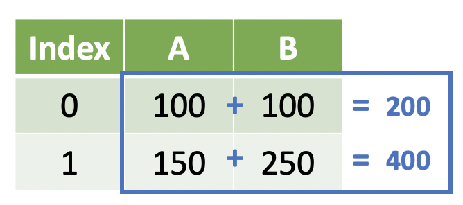
Yesterday we learned how to manipulate data across one or more variables within the row(s):
Note
We return the same number of elements that we started with. This is known as a window function, but you can also think of it as summarizing at the row-level.
We could achieve this result with the following code:
DataFrame['A'] + DataFrame['B']
We subset the two Series and then add them together using the + operator to achieve the sum.
Note that we could also use some other operation on DataFrame['B'] as long as it returns the same number of elements.
Summary Operations
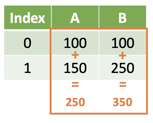
However, sometimes we want to work with data across rows within a variable -- that is, aggregate/summarize values rowwise rather than columnwise.
Note
We return a single value representing some aggregation of the elements we started with. This is known as a summary function, but you can think of it as summarizing across rows.
This is what we are going to talk about next.
Summarizing a Series
Summary Methods
The easiest way to summarize a specific series is by using bracket subsetting notation and the built-in Series methods (i.e. col.sum()):
flights_df['distance'].sum()
350217607
Note that a single value was returned because this is a summary operation -- we are summing the distance variable across all rows.
There are other summary methods with a series:
flights_df['distance'].mean()
1039.9126036297123
flights_df['distance'].median()
872.0
flights_df['distance'].std()
733.2330333236778
All of the above methods work on quantitative variables but not character variables. However, there are summary methods that will work on all types of variables:
# Number of unique values in the carrier variable
flights_df['carrier'].nunique()
16
# Most frequent value observed in the carrier variable
flights_df['carrier'].mode()
0    UA
Name: carrier, dtype: object
Your Turn
1. What is the difference between a window operation and a summary operation?
2. Fill in the blanks in the following code to calculate the mean delay in departure:
flights_df['_____']._____()
3. Find the count of each value observed in the carriers column. This may take a Google search. Would you consider the output a summary operation?
Describe Method
There is also a method describe() that provides a lot of this summary information -- this is especially useful in initial exploratory data analysis.
flights_df['distance'].describe()
count    336776.000000
mean       1039.912604
std         733.233033
min          17.000000
25%         502.000000
50%         872.000000
75%        1389.000000
max        4983.000000
Name: distance, dtype: float64
Note
The describe() method will return different results depending on the type of the Series.
flights_df['carrier'].describe()
count     336776
unique        16
top           UA
freq       58665
Name: carrier, dtype: object
Summarizing a DataFrame
The above methods and operations are nice, but sometimes we want to work with multiple variables rather than just one.
Extending Summary Methods to DataFrames
Recall how we select variables from a DataFrame:
- Single-bracket subset notation
- Pass a list of quoted variable names into the list
flights_df[['sched_dep_time', 'dep_time']]
We can use the same summary methods from the Series on the DataFrame to summarize data:
flights_df[['sched_dep_time', 'dep_time']].mean()
sched_dep_time    1344.254840
dep_time          1349.109947
dtype: float64
flights_df[['sched_dep_time', 'dep_time']].median()
sched_dep_time    1359.0
dep_time          1401.0
dtype: float64
Question
What is the type of...
flights_df[['sched_dep_time', 'dep_time']].median()?
This returns a pandas.core.series.Series object -- the Index is the variable name and the values are the summarized values.
The Aggregation Method
While summary methods can be convenient, there are a few drawbacks to using them on DataFrames:
- You have to look up or remember the method names each time
- You can only apply one summary method at a time
- You have to apply the same summary method to all variables
- A Series is returned rather than a DataFrame -- this makes it difficult to use the values in our analysis later
In order to get around these problems, the DataFrame has a powerful method agg():
flights_df.agg({
    'sched_dep_time': ['mean']
})
| sched_dep_time | |
|---|---|
| mean | 1344.25484 |
There are a few things to notice about the agg() method:
- A
dictis passed to the method with variable names as keys and a list of quoted summaries as values - A DataFrame is returned with variable names as variables and summaries as rows
Tip!
The .agg() method is just shorthand for .aggregate().
# I'm feeling quite verbose today!
flights_df.aggregate({
    'sched_dep_time': ['mean']
})
| sched_dep_time | |
|---|---|
| mean | 1344.25484 |
# I don't have that kind of time!
flights_df.agg({
    'sched_dep_time': ['mean']
})
| sched_dep_time | |
|---|---|
| mean | 1344.25484 |
We can extend this to multiple variables by adding elements to the dict:
flights_df.agg({
    'sched_dep_time': ['mean'],
    'dep_time': ['mean']
})
| sched_dep_time | dep_time | |
|---|---|---|
| mean | 1344.25484 | 1349.109947 |
And because the values of the dict are lists, we can do additional aggregations at the same time:
flights_df.agg({
    'sched_dep_time': ['mean', 'median'],
    'dep_time': ['mean', 'min']
})
| sched_dep_time | dep_time | |
|---|---|---|
| mean | 1344.25484 | 1349.109947 |
| median | 1359.00000 | NaN |
| min | NaN | 1.000000 |
Note
Not all variables have to have the same list of summaries.
Your Turn
1. What class of object is the returned by the below code?
flights_df[['air_time', 'distance']].mean()
2. What class of object is returned by the below code?
flights_df.agg({
    'air_time': ['mean'],
    'distance': ['mean']
})
3. Fill in the blanks in the below code to calculate the minimum and maximum distances traveled and the mean and median arrival delay:
flights_df.agg({
    '_____': ['min', '_____'],
    '_____': ['_____', 'median']
})
Describe Method
While agg() is a powerful method, the describe() method -- similar to the Series describe() method -- is a great choice during exploratory data analysis:
flights_df.describe()
| year | month | day | dep_time | sched_dep_time | dep_delay | arr_time | sched_arr_time | arr_delay | flight | air_time | distance | hour | minute | |
|---|---|---|---|---|---|---|---|---|---|---|---|---|---|---|
| count | 336776.0 | 336776.000000 | 336776.000000 | 328521.000000 | 336776.000000 | 328521.000000 | 328063.000000 | 336776.000000 | 327346.000000 | 336776.000000 | 327346.000000 | 336776.000000 | 336776.000000 | 336776.000000 |
| mean | 2013.0 | 6.548510 | 15.710787 | 1349.109947 | 1344.254840 | 12.639070 | 1502.054999 | 1536.380220 | 6.895377 | 1971.923620 | 150.686460 | 1039.912604 | 13.180247 | 26.230100 |
| std | 0.0 | 3.414457 | 8.768607 | 488.281791 | 467.335756 | 40.210061 | 533.264132 | 497.457142 | 44.633292 | 1632.471938 | 93.688305 | 733.233033 | 4.661316 | 19.300846 |
| min | 2013.0 | 1.000000 | 1.000000 | 1.000000 | 106.000000 | -43.000000 | 1.000000 | 1.000000 | -86.000000 | 1.000000 | 20.000000 | 17.000000 | 1.000000 | 0.000000 |
| 25% | 2013.0 | 4.000000 | 8.000000 | 907.000000 | 906.000000 | -5.000000 | 1104.000000 | 1124.000000 | -17.000000 | 553.000000 | 82.000000 | 502.000000 | 9.000000 | 8.000000 |
| 50% | 2013.0 | 7.000000 | 16.000000 | 1401.000000 | 1359.000000 | -2.000000 | 1535.000000 | 1556.000000 | -5.000000 | 1496.000000 | 129.000000 | 872.000000 | 13.000000 | 29.000000 |
| 75% | 2013.0 | 10.000000 | 23.000000 | 1744.000000 | 1729.000000 | 11.000000 | 1940.000000 | 1945.000000 | 14.000000 | 3465.000000 | 192.000000 | 1389.000000 | 17.000000 | 44.000000 |
| max | 2013.0 | 12.000000 | 31.000000 | 2400.000000 | 2359.000000 | 1301.000000 | 2400.000000 | 2359.000000 | 1272.000000 | 8500.000000 | 695.000000 | 4983.000000 | 23.000000 | 59.000000 |
Question
What is missing from the above result?
The string variables are missing!
We can make describe() compute on all variable types using the include parameter and passing a list of data types to include:
flights_df.describe(include = ['int', 'float', 'object'])
| year | month | day | dep_time | sched_dep_time | dep_delay | arr_time | sched_arr_time | arr_delay | carrier | flight | tailnum | origin | dest | air_time | distance | hour | minute | time_hour | |
|---|---|---|---|---|---|---|---|---|---|---|---|---|---|---|---|---|---|---|---|
| count | 336776.0 | 336776.000000 | 336776.000000 | 328521.000000 | 336776.000000 | 328521.000000 | 328063.000000 | 336776.000000 | 327346.000000 | 336776 | 336776.000000 | 334264 | 336776 | 336776 | 327346.000000 | 336776.000000 | 336776.000000 | 336776.000000 | 336776 |
| unique | NaN | NaN | NaN | NaN | NaN | NaN | NaN | NaN | NaN | 16 | NaN | 4043 | 3 | 105 | NaN | NaN | NaN | NaN | 6936 |
| top | NaN | NaN | NaN | NaN | NaN | NaN | NaN | NaN | NaN | UA | NaN | N725MQ | EWR | ORD | NaN | NaN | NaN | NaN | 2013-09-13 08:00:00 |
| freq | NaN | NaN | NaN | NaN | NaN | NaN | NaN | NaN | NaN | 58665 | NaN | 575 | 120835 | 17283 | NaN | NaN | NaN | NaN | 94 |
| mean | 2013.0 | 6.548510 | 15.710787 | 1349.109947 | 1344.254840 | 12.639070 | 1502.054999 | 1536.380220 | 6.895377 | NaN | 1971.923620 | NaN | NaN | NaN | 150.686460 | 1039.912604 | 13.180247 | 26.230100 | NaN |
| std | 0.0 | 3.414457 | 8.768607 | 488.281791 | 467.335756 | 40.210061 | 533.264132 | 497.457142 | 44.633292 | NaN | 1632.471938 | NaN | NaN | NaN | 93.688305 | 733.233033 | 4.661316 | 19.300846 | NaN |
| min | 2013.0 | 1.000000 | 1.000000 | 1.000000 | 106.000000 | -43.000000 | 1.000000 | 1.000000 | -86.000000 | NaN | 1.000000 | NaN | NaN | NaN | 20.000000 | 17.000000 | 1.000000 | 0.000000 | NaN |
| 25% | 2013.0 | 4.000000 | 8.000000 | 907.000000 | 906.000000 | -5.000000 | 1104.000000 | 1124.000000 | -17.000000 | NaN | 553.000000 | NaN | NaN | NaN | 82.000000 | 502.000000 | 9.000000 | 8.000000 | NaN |
| 50% | 2013.0 | 7.000000 | 16.000000 | 1401.000000 | 1359.000000 | -2.000000 | 1535.000000 | 1556.000000 | -5.000000 | NaN | 1496.000000 | NaN | NaN | NaN | 129.000000 | 872.000000 | 13.000000 | 29.000000 | NaN |
| 75% | 2013.0 | 10.000000 | 23.000000 | 1744.000000 | 1729.000000 | 11.000000 | 1940.000000 | 1945.000000 | 14.000000 | NaN | 3465.000000 | NaN | NaN | NaN | 192.000000 | 1389.000000 | 17.000000 | 44.000000 | NaN |
| max | 2013.0 | 12.000000 | 31.000000 | 2400.000000 | 2359.000000 | 1301.000000 | 2400.000000 | 2359.000000 | 1272.000000 | NaN | 8500.000000 | NaN | NaN | NaN | 695.000000 | 4983.000000 | 23.000000 | 59.000000 | NaN |
Questions
Are there any questions before we move on?