Introduction to Machine Learning
Introduction
Machine learning (ML) continues to grow in importance for many organizations across nearly all domains. Some example applications of machine learning in practice include:
- Predicting the likelihood of a patient returning to the hospital (readmission) within 30 days of discharge.
- Segmenting customers based on common attributes or purchasing behavior for targeted marketing.
- Predicting coupon redemption rates for a given marketing campaign.
- Predicting customer churn so an organization can perform preventative intervention.
- And many more!
To address each scenario, we can use a given set of features to train an algorithm and extract insights.
Types of modeling
These algorithms, or learners, can be classified according to the amount and type of supervision needed during training.
Two primary categories of algorithms:
- ___supervised learners___ which construct predictive models
- ___unsupervised learners___ which build descriptive models.
Which type you will need to use depends on the learning task you hope to accomplish.
Supervised learning
A ___predictive model___ is used for tasks that involve the prediction of a given output (or target) using other variables (or features) in the data set.
The learning algorithm in a predictive model attempts to discover and model the relationships among the target variable (the variable being predicted) and the other features (aka predictor variables).
Examples of predictive modeling include:
- using customer attributes to predict the probability of the customer churning in the next 6 weeks;
- using home attributes to predict the sales price;
- using employee attributes to predict the likelihood of attrition;
- using patient attributes and symptoms to predict the risk of readmission;
- using production attributes to predict time to market.
Types of supervised learning
Most supervised learning problems can be bucketed into one of two categories, regression or classification
- Regression: objective is to predict a numeric outcome
- What is the expected sales price?
- What is the expected wait time?
- What is the expected time to market?
- Classification: objective is to predict a categorical outcome
- Did a customer redeem a coupon (coded as yes/no or 1/0)?
- Did a customer churn (coded as yes/no or 1/0)?
- Did a customer click on our online ad (coded as yes/no or 1/0)?
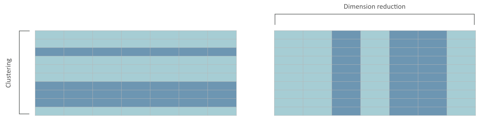
Unsupervised learning
A set of statistical tools to better understand n observations that contain a set of features without being guided by a response variable.
In essence, unsupervised learning is concerned with identifying groups in a data set
- clustering: reduce the observation space of a data set
- dimension reduction: reduce the feature space of a data set
Today's focus
Supervised learning for a regression problem
using home attributes to predict real estate sales price
Objective: understand the basic supervised learning modeling process and how to implement with scikit-learn
Our ___Advanced Python workshop___ will go into much more detail than we have time for here.
Supervised learning modeling process
Modeling Process
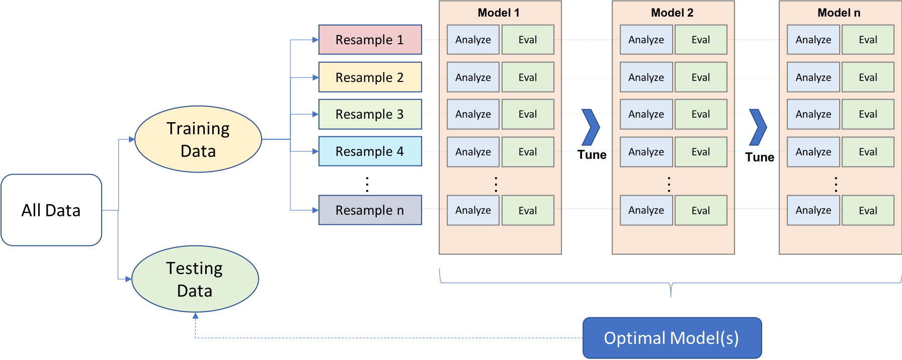
The machine learning process is very iterative and heurstic-based
Common for many ML approaches to be applied, evaluated, and modified before a final, optimal model can be determined
A proper process needs to be implemented to have confidence in our results
Modeling Process
This module provides an introduction to the modeling process and the concepts that are useful for any type of machine learning model:
data splitting
model application
resampling
bias-variance trade-off -- hyperparameter tuning
model evaluation
Prerequisites - packages
# Helper packages
import math
import numpy as np
import pandas as pd
from plotnine import (
    ggplot, aes, geom_density,
    geom_line, geom_point, ggtitle
)

# Modeling process
from sklearn.model_selection import (
    train_test_split, KFold, RepeatedKFold, cross_val_score
)
from sklearn.model_selection import GridSearchCV
from sklearn.metrics import mean_squared_error
Prerequisites - Ames housing data
- problem type: supervised regression
- response variable:
Sale_Price(i.e., \$195,000, \$215,000) - features: 80
- observations: 2,930
- objective: use property attributes to predict the sale price of a home
# Ames housing data
ames = pd.read_csv("../data/ames.csv")
ames.head()
| MS_SubClass | MS_Zoning | Lot_Frontage | Lot_Area | Street | Alley | Lot_Shape | Land_Contour | Utilities | Lot_Config | ... | Fence | Misc_Feature | Misc_Val | Mo_Sold | Year_Sold | Sale_Type | Sale_Condition | Sale_Price | Longitude | Latitude | |
|---|---|---|---|---|---|---|---|---|---|---|---|---|---|---|---|---|---|---|---|---|---|
| 0 | One_Story_1946_and_Newer_All_Styles | Residential_Low_Density | 141 | 31770 | Pave | No_Alley_Access | Slightly_Irregular | Lvl | AllPub | Corner | ... | No_Fence | NaN | 0 | 5 | 2010 | WD | Normal | 215000 | -93.619754 | 42.054035 |
| 1 | One_Story_1946_and_Newer_All_Styles | Residential_High_Density | 80 | 11622 | Pave | No_Alley_Access | Regular | Lvl | AllPub | Inside | ... | Minimum_Privacy | NaN | 0 | 6 | 2010 | WD | Normal | 105000 | -93.619756 | 42.053014 |
| 2 | One_Story_1946_and_Newer_All_Styles | Residential_Low_Density | 81 | 14267 | Pave | No_Alley_Access | Slightly_Irregular | Lvl | AllPub | Corner | ... | No_Fence | Gar2 | 12500 | 6 | 2010 | WD | Normal | 172000 | -93.619387 | 42.052659 |
| 3 | One_Story_1946_and_Newer_All_Styles | Residential_Low_Density | 93 | 11160 | Pave | No_Alley_Access | Regular | Lvl | AllPub | Corner | ... | No_Fence | NaN | 0 | 4 | 2010 | WD | Normal | 244000 | -93.617320 | 42.051245 |
| 4 | Two_Story_1946_and_Newer | Residential_Low_Density | 74 | 13830 | Pave | No_Alley_Access | Slightly_Irregular | Lvl | AllPub | Inside | ... | Minimum_Privacy | NaN | 0 | 3 | 2010 | WD | Normal | 189900 | -93.638933 | 42.060899 |
5 rows × 81 columns
Your Turn
Take 5 minutes to explore the housing data
What does the distribution of the response variable (
Sale_Price) look like?How could the different features be helpful in predicting the sales price?
Data Splitting
Generalizability
Generalizability: we want an algorithm that not only fits well to our past data, but more importantly, one that predicts a future outcome accurately.
Training Set: these data are used to develop feature sets, train our algorithms, tune hyper-parameters, compare across models, and all of the other activities required to reach a final model decision.
Test Set: having chosen a final model, these data are used to estimate an unbiased assessment of the model’s performance (generalization error).

DO NOT TOUCH THE TEST SET UNTIL THE VERY END!!!
What's the right split?
typical recommendations for splitting your data into training-testing splits include 60% (training) - 40% (testing), 70%-30%, or 80%-20%
as data sets get smaller ($n < 500$):
- spending too much in training ($> 80$%) won’t allow us to get a good assessment of predictive performance. We may find a model that fits the training data very well, but is not generalizable (overfitting),
- sometimes too much spent in testing ($> 40$%) won’t allow us to get a good assessment of model parameters
as n gets larger ($n > 100$K):
- marginal gains with larger sample sizes
- may use a smaller training sample to increase computation speed
as p gets larger ($p \geq n$)
- larger samples sizes are often required to identify consistent signals in the features
Mechanics of data splitting
# create train/test split
train, test = train_test_split(ames, train_size=0.7, random_state=123)
# dimensions of training data
train.shape
(2051, 81)
# dimensions of testing data
test.shape
(879, 81)
Visualizing response distribution
Always good practice to ensure the distribution of our target variable is similar across the training and test sets
(ggplot(train, aes(x='Sale_Price'))
 + geom_density(color='blue')
 + geom_density(data = test, color = "red")
 + ggtitle("Distribution of Sale_Price"))

<Figure Size: (640 x 480)>
Separating features & target
In Python, we are required to separate our features from our label into discrete data sets.
For our first model we will simply use two features from our training data - total square feet of the home (
Gr_Liv_Area) and year built (Year_Built) to predict the sale price.
# separate features from labels
X_train = train[["Gr_Liv_Area", "Year_Built"]]
y_train = train["Sale_Price"]
Creating Models
Creating Models with scikit-learn
Scikit-learn has many modules for supervised learning
- Linear models (i.e. ordinary least squares)
- Nearest neighbors (i.e. K-nearest neighbor)
- Tree-based models (i.e. decision trees, random forests)
- and many more: https://scikit-learn.org/stable/supervised_learning.html
To apply these models, they all follow a similar pattern:
- Identify the appropriate module
- Instantiate the model object
- Fit the model
- Make predictions
Ordinary least squares
# 1. Prerequisite
from sklearn.linear_model import LinearRegression
# 2. Instantiate the model object
reg = LinearRegression()
# 3. Fit the model
reg.fit(X_train, y_train)
LinearRegression()In a Jupyter environment, please rerun this cell to show the HTML representation or trust the notebook.
On GitHub, the HTML representation is unable to render, please try loading this page with nbviewer.org.
LinearRegression()
# 4. Make predictions
reg.predict(X_train)
array([211888.77551558, 119021.83893513, 177818.03700616, ...,
       294633.08255954, 213774.91574325, 166398.33102108])
K-nearest neighhbor
# 1. Prerequisite
from sklearn.neighbors import KNeighborsRegressor
# 2. Instantiate the model object
knn = KNeighborsRegressor()
# 3. Fit the model
knn.fit(X_train, y_train)
KNeighborsRegressor()In a Jupyter environment, please rerun this cell to show the HTML representation or trust the notebook.
On GitHub, the HTML representation is unable to render, please try loading this page with nbviewer.org.
KNeighborsRegressor()
# 4. Make predictions
knn.predict(X_train)
array([218400. , 131280. , 142600. , ..., 318647.2, 180820. , 149480. ])
Your Turn
Create and predict a model using the random forest algorithm.
# 1. Prerequisite
from sklearn.ensemble import RandomForestRegressor
# 2. Instantiate the model object
rf = RandomForestRegressor()
# 3. Fit the model
rf.fit(X_train, y_train)
RandomForestRegressor()In a Jupyter environment, please rerun this cell to show the HTML representation or trust the notebook.
On GitHub, the HTML representation is unable to render, please try loading this page with nbviewer.org.
RandomForestRegressor()
# 4. Make predictions
rf.predict(X_train)
array([171438.        , 118076.        , 142605.42388167, ...,
       286305.        , 194271.98133333, 135037.48      ])
Evaluating Models
Evaluating model performance
It is important to understand how our model is performing.
With ML models, measuring performance means understanding the predictive accuracy -- the difference between a predicted value and the actual value.
We measure predictive accuracy with ___loss functions___.
Many loss functions for regression problems
- Mean Square Error (MSE) = $\frac{1}{n} \sum^n_{i=1} (y_i - \hat{y}_i)^2$
- Root Mean Square Error (RMSE) = $\sqrt{MSE}$
- Other common loss functions
- Mean Absolute Error (MAE)
- Mean Absolute Percent Error (MAPE)
- Root Mean Squared Logarithmic Error (RMSLE)
Computing MSE
# compute MSE for linear model
pred = reg.predict(X_train)
mse = mean_squared_error(y_train, pred)
mse
2313058425.399425
rmse = math.sqrt(mse)
rmse
48094.2660345225
On average, our model's predictions are over \$48,000 off from the actual sales price!!
Your Turn
With MSE & RMSE our objective is to ___minimize___ this value.
Compare the MSE & RMSE for the K-nearest neighbor and random forest model to our linear model.
Which model performs best?
Are we certain this is the best way to measure our models' performance?
Resampling Methods
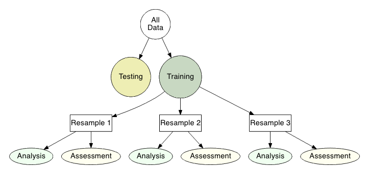
Resampling methods
Provides an approach for us to repeatedly fit a model of interest to parts of the training data and test the performance on other parts.
Allows us to estimate the generalization error while training, tuning, and comparing models without using the test data set
The two most commonly used resampling methods include:
- k-fold cross validation
- bootstrapping.
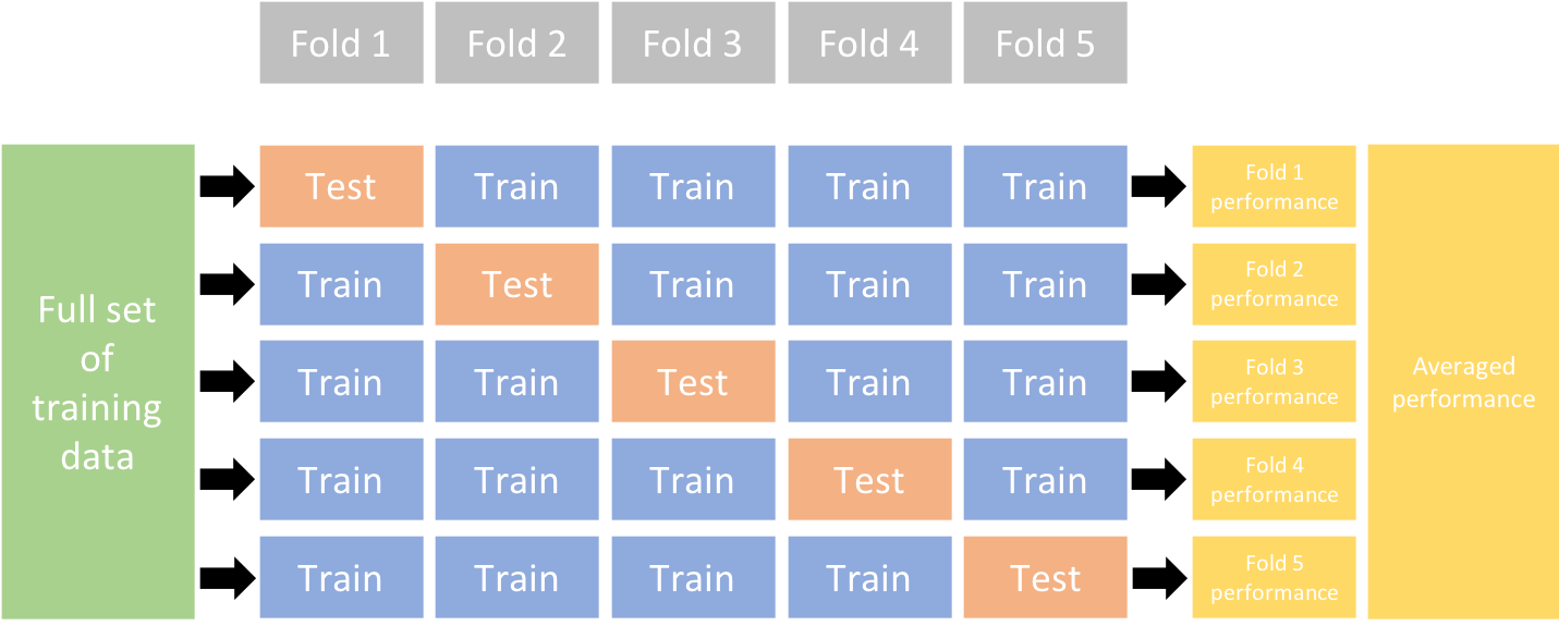
K-fold cross validation
randomly divides the training data into k groups of approximately equal size
assign one block as the test block and the rest as training block
train model on each folds' training block and evaluate on test block
average performance across all folds
K-fold CV implementation
- Use
KFoldto create k-fold objects and then cross_val_scoreto train our model across all k folds and provide our loss score for each fold
# define loss function
loss = 'neg_root_mean_squared_error'

# create 10 fold CV object
kfold = KFold(n_splits=10, random_state=123, shuffle=True)

# fit KNN model with 10-fold CV
results = cross_val_score(
    knn, X_train, y_train, cv=kfold, scoring=loss
)
results
array([-44371.6172573 , -40053.49695081, -52321.53768451, -46339.69606634,
       -45736.42785737, -53089.81175919, -42830.25107754, -45540.49867468,
       -48512.75628167, -58652.48566654])
Note: The unified scoring API in scikit-learn always maximizes the score, so scores which need to be minimized are negated in order for the unified scoring API to work correctly. Consequently, you can just interpret the RMSE values below as the $RMSE \times -1$.
K-fold results
# summary stats for all 10 folds
pd.DataFrame(results * -1).describe()
| 0 | |
|---|---|
| count | 10.000000 |
| mean | 47744.857928 |
| std | 5524.060076 |
| min | 40053.496951 |
| 25% | 44663.837612 |
| 50% | 46038.061962 |
| 75% | 51369.342334 |
| max | 58652.485667 |
Your Turn
Compute K-fold results for the linear model and/or the random forest model.
How do the results compare?
Hyperparameter Tuning
Bias-variance trade-off
Prediction errors can be decomposed into two main subcomponents we have control over:
- error due to “bias”
- error due to “variance”
There is a tradeoff between a model’s ability to minimize bias and variance.
Understanding how different sources of error lead to bias and variance helps us improve the data fitting process resulting in more accurate models.
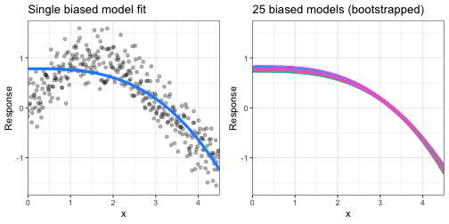
Bias
Bias is the difference between the expected (or average) prediction of our model and the correct value which we are trying to predict.
Some models are naturally ___high bias___:
- Models that are not very flexible (i.e. generalized linear models)
- High bias models are rarely affected by the noise introduced by resampling
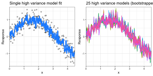
Variance
Error due to ___variance___ is defined as the variability of a model prediction for a given data point.
Some models are naturally high variance:
- Models that are very adaptable and offer extreme flexibility in the patterns that they can fit to (e.g., k-nearest neighbor, decision trees, gradient boosting machines).
- These models offer their own problems as they run the risk of overfitting to the training data.
- Although you may achieve very good performance on your training data, the model will not automatically generalize well to unseen data.
Hyperparameter tuning
So what does this mean to you?
- We tend to like very flexible models since they can capture many patterns in our data,
- but we need to control variance so our model generalizes to new data well.
- ___Hyperparameters___ can help to control bias-variance trade-off
Hyperparameter tuning
Hyperparameters are the "knobs to twiddle" to control of complexity of machine learning algorithms and, therefore, the bias-variance trade-off
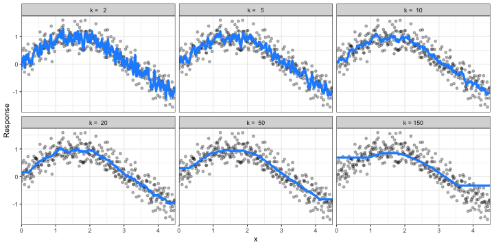
k-nearest neighbor model with differing values for k. Small k value has too much variance. Big k value has too much bias. How do we find the optimal value?
Grid search
A grid search is an automated approach to searching across many combinations of hyperparameter values
We perform a grid search with
GridSearchCV()and supply it a model object and hyperparameter values we want to assess.Also notice that we supply it with the
kfoldobject we created previously and thelossfunction we want to optimize for.
# Basic model object
knn = KNeighborsRegressor()

# Hyperparameter values to assess
hyper_grid = {'n_neighbors': range(2, 26)}

# Create grid search object
grid_search = GridSearchCV(knn, hyper_grid, cv=kfold, scoring=loss)

# Tune a knn model using grid search
results = grid_search.fit(X_train, y_train)
# Best model's cross validated RMSE
abs(results.best_score_)
46651.2105708044
# Best model's k value
results.best_estimator_.get_params().get('n_neighbors')
13
# Plot all RMSE results
all_rmse = pd.DataFrame({
    'k': range(2, 26),
    'RMSE': np.abs(results.cv_results_['mean_test_score'])
})

(ggplot(all_rmse, aes(x='k', y='RMSE'))
 + geom_line()
 + geom_point()
 + ggtitle("Cross validated grid search results"))

<Figure Size: (640 x 480)>
Putting the Processes Together
Putting the Processes Together
You've been exposed to a lot in a very short amount of time. Let's bring these pieces together but rather than just look at the 2 features that we included thus far (Gr_Liv_Area & Year_Built), we'll include ___all numeric features___.
Steps:
Split into training vs testing data
Separate features from labels and only use numeric features
Create KNN model object
Define loss function
Specify K-fold resampling procedure
Create our hyperparameter grid
Execute grid search
Evaluate performance
# 1. Split into training vs testing data
train, test = train_test_split(ames, train_size=0.7, random_state=123)

# 2. Separate features from labels and only use numeric features
X_train = (
    train.select_dtypes(include='number').drop("Sale_Price", axis=1)
)
y_train = train["Sale_Price"]

# 3. Create KNN model object
knn = KNeighborsRegressor()

# 4. Define loss function
loss = 'neg_root_mean_squared_error'

# 5. Specify K-fold resampling procedure
kfold = KFold(n_splits=10, random_state=123, shuffle=True)

# 6. Create grid of hyperparameter values
hyper_grid = {'n_neighbors': range(2, 26)}

# 7. Tune a knn model using grid search
grid_search = GridSearchCV(knn, hyper_grid, cv=kfold, scoring=loss)
results = grid_search.fit(X_train, y_train)
# 8. Evaluate performance: Best model's cross validated RMSE
abs(results.best_score_)
41915.408581298376
# 8. Evaluate performance: Best model's k value
results.best_estimator_.get_params().get('n_neighbors')
5
# 8. Evaluate performance: Plot all RMSE results
all_rmse = pd.DataFrame({
    'k': range(2, 26),
    'RMSE': np.abs(results.cv_results_['mean_test_score'])
})

(ggplot(all_rmse, aes(x='k', y='RMSE'))
 + geom_line()
 + geom_point()
 + ggtitle("Cross validated grid search results"))

<Figure Size: (640 x 480)>
Can we do better?
Is this the best we can do?
Do you think other models could perform better?
Are we doing the best with the features we've been given?
Learning More
- Don't feel intimated -- you're not going to learn this in an hour
- There are a lot of things you can do to improve your skills
- Books
- Introduction to Statistical Learning or Elements of Statistical Learning, Hastie, Tibshirani, and Friedman
- Python Data Science Handbook, Jake VanderPlas
- Hands-on Machine Learning with scikit-learn and TensorFlow, Aurélien Géron
- Online Courses
- Machine Learning with Python - Coursera
- Practice
- Use your own data
- Kaggle
Questions
Are there any questions before moving on?