
Basic, Important Data Structures
- Python has a few key built-in data structures
- The two most important for what we will talk about are the list and the dictionary
The List
- Python's
liststructure is a very important one-dimensional data structure
- It is created with single brackets
[]or by calling thelist()function
In [1]:
a_list = [1, 2, 3]
a_list
Out[1]:
[1, 2, 3]
- And a
listcan be subset using single-bracket notation -- note that they index from 0
In [2]:
a_list[0]
Out[2]:
1
The Dictionary
- Python
dictstructure is a popular way of representing key-value pairs
- It is created with braces
{}or by calling thedict()function
In [3]:
a_dict = {
    'key1': 'value1',
    'key2': 2,
    'key3': [1, 2, 3]
}
- A
dictcan be subset using single-bracket notation and a key value:
In [4]:
a_dict['key1']
Out[4]:
'value1'
pandas is Important...
- The
pandasPython package is the most popular choice of working with tabular data in Python
- We covered a lot of
pandasbasics in the Introduction to Python for Data Science class
- Due to their importance to this class and data science in Python, we're going to do a (very) quick whirlwind of the key points
pandasis commonly imported as:
In [5]:
import pandas as pd
The pandas DataFrame
- The
pandasDataFrame class is the most popular choice to represent tabular data in Python
- DataFrames are two-dimensional -- similar to a common spreadsheet, table or dataset
- DataFrames have attributes (data) and methods (operations) to provide useful information via dot-notation
DataFrame.head()is a method that shows the first 5 rows of a DataFrameDataFrame.shapeis an attribute that displays the number of rows and number of variables of a DataFrame
Importing DataFrames
- Tabular data can be imported to DataFrames from a variety of sources:
- Delimited files
- JSON or similar files
- Database connections
- Spark DataFrames
- For this class, we'll be working with delimited files like CSVs
Importing DataFrames from Delimited Files
- Delimited files can be imported into DataFrames using the
pd.read_csv()function:
In [6]:
planes_df = pd.read_csv('../data/planes.csv')
planes_df.head()
Out[6]:
| tailnum | year | type | manufacturer | model | engines | seats | speed | engine | |
|---|---|---|---|---|---|---|---|---|---|
| 0 | N10156 | 2004.0 | Fixed wing multi engine | EMBRAER | EMB-145XR | 2 | 55 | NaN | Turbo-fan |
| 1 | N102UW | 1998.0 | Fixed wing multi engine | AIRBUS INDUSTRIE | A320-214 | 2 | 182 | NaN | Turbo-fan |
| 2 | N103US | 1999.0 | Fixed wing multi engine | AIRBUS INDUSTRIE | A320-214 | 2 | 182 | NaN | Turbo-fan |
| 3 | N104UW | 1999.0 | Fixed wing multi engine | AIRBUS INDUSTRIE | A320-214 | 2 | 182 | NaN | Turbo-fan |
| 4 | N10575 | 2002.0 | Fixed wing multi engine | EMBRAER | EMB-145LR | 2 | 55 | NaN | Turbo-fan |
- There are many parameters associated with
pd.read_csv(), likesep, to customize the importing based on your data
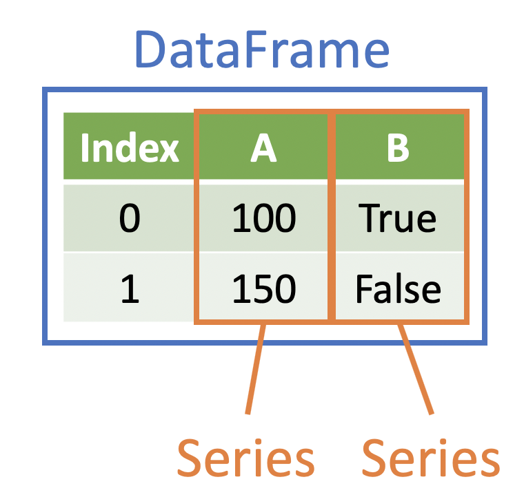
DataFrame Structure
DataFrames are made up of Series
- DataFrame variables are objects known as Series
- A DataFrame can be thought of as a list of equal-length Series
- As you work with DataFrames in more complex and efficient ways, the Series can become increasingly important
All DataFrames have an Index
- Every DataFrame has something called an Index which is similar to a column
- When printing DataFrames in Jupyter, the Index is visible on the far-left side of the DataFrame
- By default, the Index value for each row is equal to the row number (starting at zero)
In [7]:
planes_df.head(2)
Out[7]:
| tailnum | year | type | manufacturer | model | engines | seats | speed | engine | |
|---|---|---|---|---|---|---|---|---|---|
| 0 | N10156 | 2004.0 | Fixed wing multi engine | EMBRAER | EMB-145XR | 2 | 55 | NaN | Turbo-fan |
| 1 | N102UW | 1998.0 | Fixed wing multi engine | AIRBUS INDUSTRIE | A320-214 | 2 | 182 | NaN | Turbo-fan |
- However, the Index can be changed -- it's common to make a column the Index
Subsetting DataFrames
- Recall that DataFrames are two-dimensional
- Therefore, DataFrames can be subset in two ways:
- Column/Variable - limiting the number of columns/variables, which is known as selecting
- Rows/Cases - limiting the number of rows/cases, which is known as filtering or slicing
Selecting DataFrame Variables
- Recall that DataFrame columns/variables are Series
- A DataFrame variable can be seleted as a Series using single-bracket notation and the quoted name of the variable:
In [8]:
planes_df['model'].head()
Out[8]:
0    EMB-145XR
1     A320-214
2     A320-214
3     A320-214
4    EMB-145LR
Name: model, dtype: object
- In order to select the variable as a DataFrame, a list of the quoted name of the variable must be provided:
In [9]:
planes_df[['model']].head(3)
Out[9]:
| model | |
|---|---|
| 0 | EMB-145XR |
| 1 | A320-214 |
| 2 | A320-214 |
- This allows multiple variables to be selected:
In [10]:
planes_df[['model', 'engines']].head(3)
Out[10]:
| model | engines | |
|---|---|---|
| 0 | EMB-145XR | 2 |
| 1 | A320-214 | 2 |
| 2 | A320-214 | 2 |
Filtering DataFrame Rows
- DataFrame rows can be filtered by providing a logical condition equal-in-length to the number of rows in the DataFrame
- Rows where the logical condition is
Truewill be returned and rows where the logical condition isFalsewill be removed
In [11]:
planes_df['year'].head()
Out[11]:
0    2004.0
1    1998.0
2    1999.0
3    1999.0
4    2002.0
Name: year, dtype: float64
In [12]:
(planes_df['year'] >= 2000).head()
Out[12]:
0     True
1    False
2    False
3    False
4     True
Name: year, dtype: bool
In [13]:
planes_df.loc[planes_df['year'] >= 2000].head(2)
Out[13]:
| tailnum | year | type | manufacturer | model | engines | seats | speed | engine | |
|---|---|---|---|---|---|---|---|---|---|
| 0 | N10156 | 2004.0 | Fixed wing multi engine | EMBRAER | EMB-145XR | 2 | 55 | NaN | Turbo-fan |
| 4 | N10575 | 2002.0 | Fixed wing multi engine | EMBRAER | EMB-145LR | 2 | 55 | NaN | Turbo-fan |
Manipulating DataFrame Columns
- When working with DataFrame columns, we're working with Series
- So DataFrame column operations are really Series operations
Manipulating Existing Columns
- An existing column can be overwritten by subsetting the Series, manipulating the Series, and then reassigning the the Series:
In [14]:
planes_df['type'] = planes_df['type'].str.upper()
planes_df['type'].head()
Out[14]:
0    FIXED WING MULTI ENGINE
1    FIXED WING MULTI ENGINE
2    FIXED WING MULTI ENGINE
3    FIXED WING MULTI ENGINE
4    FIXED WING MULTI ENGINE
Name: type, dtype: object
Creating New Columns
- A new column can be created by assigning an object equal to the number of rows in the DataFrame to a newly-named Series:
In [15]:
planes_df['seats_and_crew'] = planes_df['seats'] + 5
planes_df[['seats', 'seats_and_crew']].head()
Out[15]:
| seats | seats_and_crew | |
|---|---|---|
| 0 | 55 | 60 |
| 1 | 182 | 187 |
| 2 | 182 | 187 |
| 3 | 182 | 187 |
| 4 | 55 | 60 |
Summarizing DataFrames
- Recall that summarizing data is the process of summarizing many rows of data into a single row of data
- There are a variety of methods that can be used to summarize the data in DataFrames
Simple Summaries
- Built-in summary methods are useful for summarizing Series
In [16]:
planes_df['seats'].mean()
Out[16]:
154.31637567730283
- These built-in summaries also work for DataFrames
In [17]:
planes_df.mean(numeric_only=True)
Out[17]:
year              2000.484010
engines              1.995184
seats              154.316376
speed              236.782609
seats_and_crew     159.316376
dtype: float64
Flexible Summaries
- The
agg()method provides more flexibility when summarizing DataFrames
agg()accepts adictargument with column-name keys and alistof summary functions as values
In [18]:
planes_df.agg({
    'seats': ['mean'],
    'engines': ['max', 'min']
})
Out[18]:
| seats | engines | |
|---|---|---|
| mean | 154.316376 | NaN |
| max | NaN | 4.0 |
| min | NaN | 1.0 |
Grouped Summaries
- Before summarizing, DataFrames can be grouped by a variable using the
groupby()method
In [19]:
(
    planes_df.groupby('manufacturer', as_index = False)
    .agg({'seats': ['mean']}).head()
)
Out[19]:
| manufacturer | seats | |
|---|---|---|
| mean | ||
| 0 | AGUSTA SPA | 8.000000 |
| 1 | AIRBUS | 221.202381 |
| 2 | AIRBUS INDUSTRIE | 187.402500 |
| 3 | AMERICAN AIRCRAFT INC | 2.000000 |
| 4 | AVIAT AIRCRAFT INC | 2.000000 |
Combining DataFrames
- Because DataFrames are two-dimensional, they can be combined both vertically and horizontally
Combining Vertically
- Combining DataFrames vertically is usually referred to as appending or unioning
- It is simply stacking DataFrames on top of one another
- The
concat()function is used to union a list of DataFrames
In [20]:
df_1 = pd.DataFrame({'a': [100, 200]})
df_2 = pd.DataFrame({'a': [300, 400]})
pd.concat([df_1, df_2]).reset_index(drop = True)
Out[20]:
| a | |
|---|---|
| 0 | 100 |
| 1 | 200 |
| 2 | 300 |
| 3 | 400 |
Combining Horizontally
- Combining DataFrames horizontally is usually referred to as joining or merging
- Joining/merging occurs using a key column that is present in both DataFrames being combined -- this is used to align the rows
- The
merge()function is used to join DataFrames
In [21]:
flights_df = pd.read_csv('../data/flights.csv')
pd.merge(flights_df, planes_df, how = 'left', on = 'tailnum').head(2)
Out[21]:
| year_x | month | day | dep_time | sched_dep_time | dep_delay | arr_time | sched_arr_time | arr_delay | carrier | ... | time_hour | year_y | type | manufacturer | model | engines | seats | speed | engine | seats_and_crew | |
|---|---|---|---|---|---|---|---|---|---|---|---|---|---|---|---|---|---|---|---|---|---|
| 0 | 2013 | 1 | 1 | 517.0 | 515 | 2.0 | 830.0 | 819 | 11.0 | UA | ... | 2013-01-01 05:00:00 | 1999.0 | FIXED WING MULTI ENGINE | BOEING | 737-824 | 2.0 | 149.0 | NaN | Turbo-fan | 154.0 |
| 1 | 2013 | 1 | 1 | 533.0 | 529 | 4.0 | 850.0 | 830 | 20.0 | UA | ... | 2013-01-01 05:00:00 | 1998.0 | FIXED WING MULTI ENGINE | BOEING | 737-824 | 2.0 | 149.0 | NaN | Turbo-fan | 154.0 |
2 rows × 28 columns
Questions
Are there any questions before we move on?